Period and analysis charts
The Period Chart object shows one bar per hour, day or month: energy, uptime, average, maximum or minimum, with monthly targets. The Analysis Chart object shows statistics of a time range, such as a histogram or a heatmap.
Before you begin
- The page is open in the screen editor.
- The signals are recorded in an archive table; see Archive tables and assignments. Both objects read the history, so a period older than the retention of the table or a time before the recording started stays empty.
Steps
1. Place a Period Chart
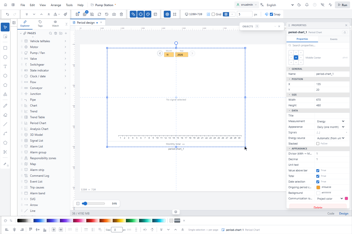
In WIDGETS, click Period Chart and draw a rectangle on the page. All fields are listed in Period Chart.
2. Choose the measurement and the signals
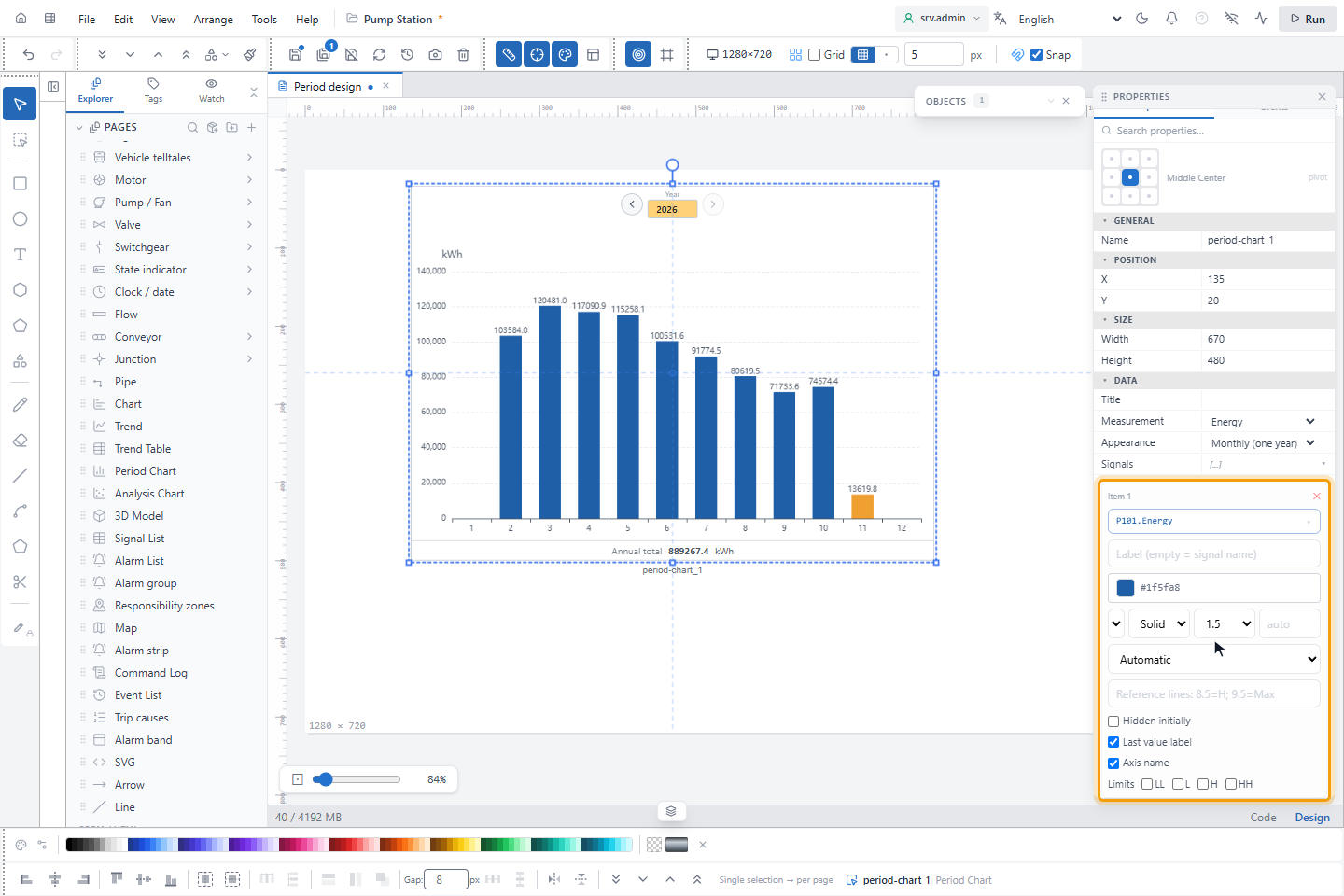
Set Appearance to Hourly (one day), Daily (one month) or Monthly (one year) and Measurement to what each bar shows:
| Measurement | Each bar | Required fields |
|---|---|---|
| Energy | Energy of the period, see below | Signals, one meter or power signal per pen. Stacked stacks the pens and writes the total above them. |
| Uptime | Running hours in the period | Power signal and Power threshold (above = running). Optional Breaker signal with Breaker closed value. |
| Average | Average of the hourly averages | Signals |
| Maximum, Minimum | Highest or lowest value in the period | Signals |
Energy source decides how energy is calculated:
| Energy source | For | Energy of a period |
|---|---|---|
| Meter (kWh / MWh) | A cumulative meter | End of the period minus end of the previous period |
| Power (kW / MW) | Instantaneous power | Average power of each hour × 1 hour |
| Automatic (from unit) | Both | A unit ending in Wh, VAh or varh is a meter, a unit ending in W, VA or var is power, any other unit is a meter |
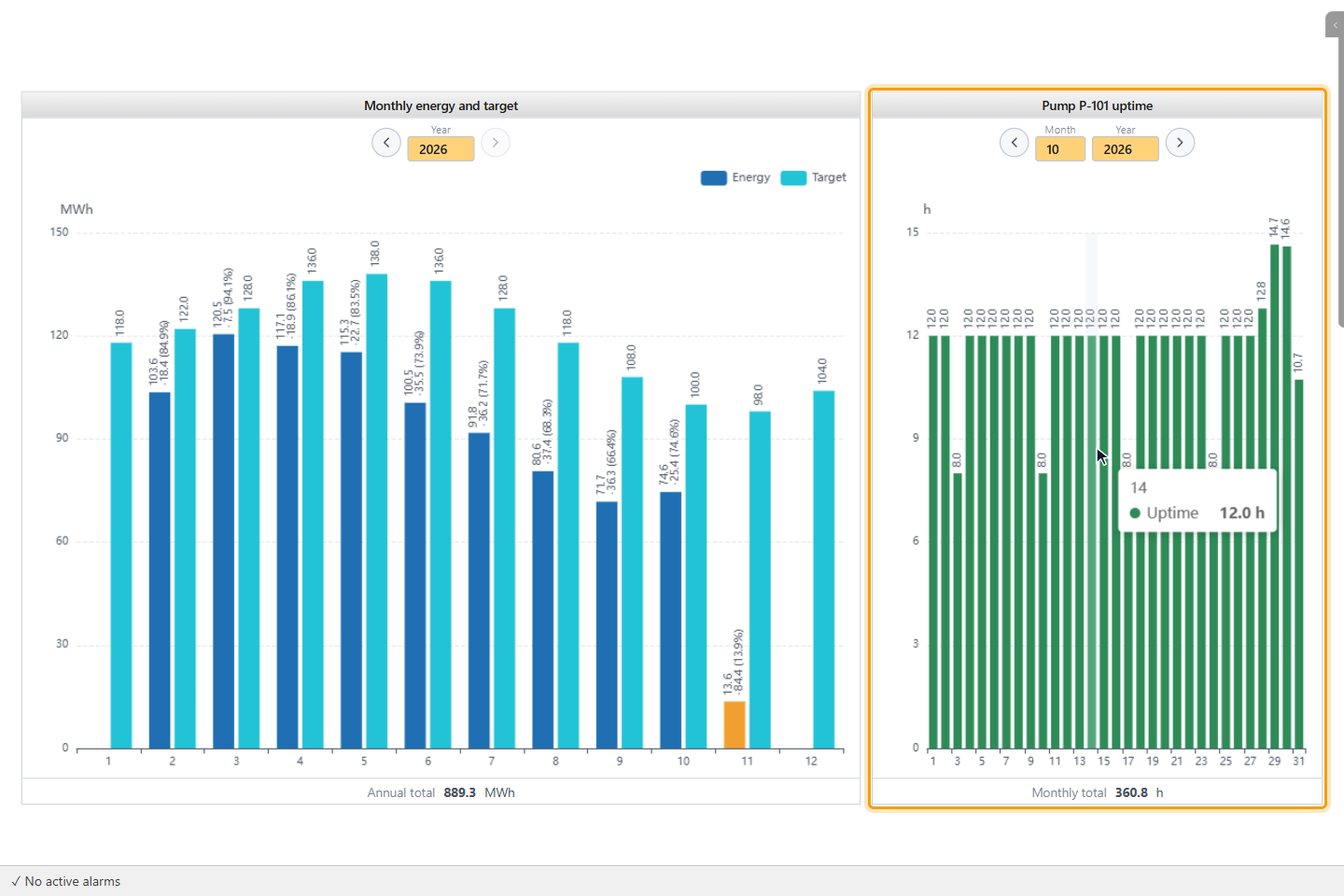
For Uptime, a period counts as running while the power is above the threshold and the breaker is closed. Without a breaker signal only the power counts. YTCC works from hourly values, so an hour in which the state changes is an approximation.
Under APPEARANCE, Divisor (kWh → MWh: 1000), Decimal and Unit text format the values, and Value above bar, Total and Date selection show or hide these parts.
3. Enter the monthly targets
With Appearance on Monthly (one year), expand Monthly target. Choose Shared (every year) or a year, and type a value for the months 1 to 12. A year without its own targets uses the shared ones. The values are in the unit of the signal, before Divisor (kWh → MWh: 1000). The ✕ next to the year (Delete this year's targets) removes them.
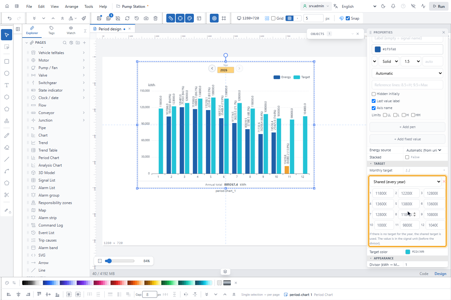
Targets are shown only in the monthly view and not with Uptime.
4. Read the chart on the run screen
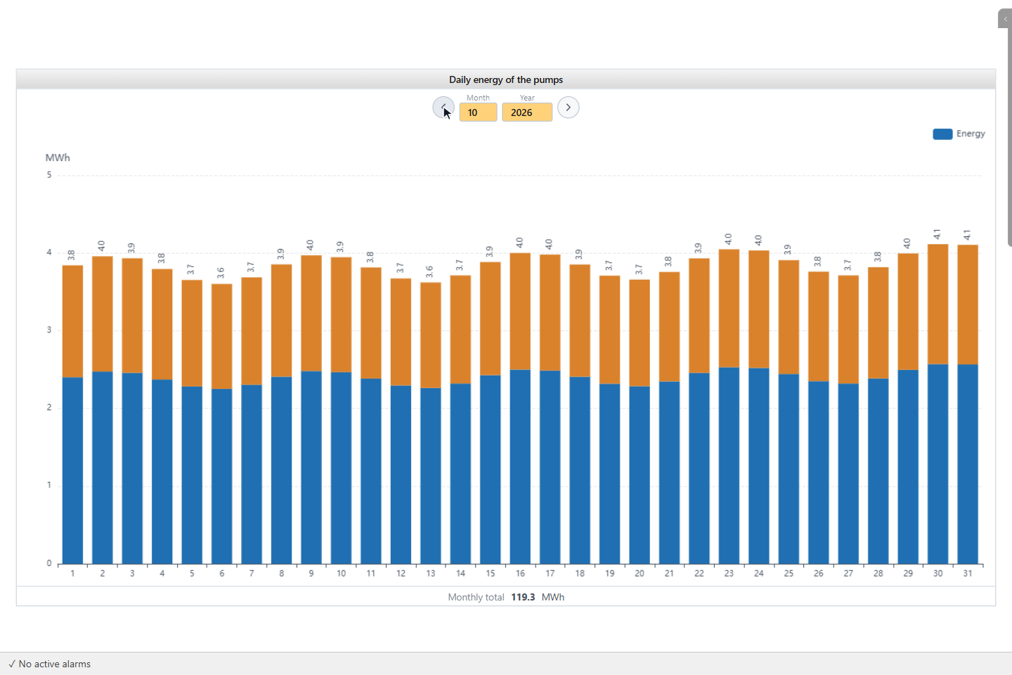
Save the page and open it on the run screen. The arrows Previous and Next and the boxes Day, Month and Year choose the period in the calendar of the browser. Next is off when the shown period is still running.
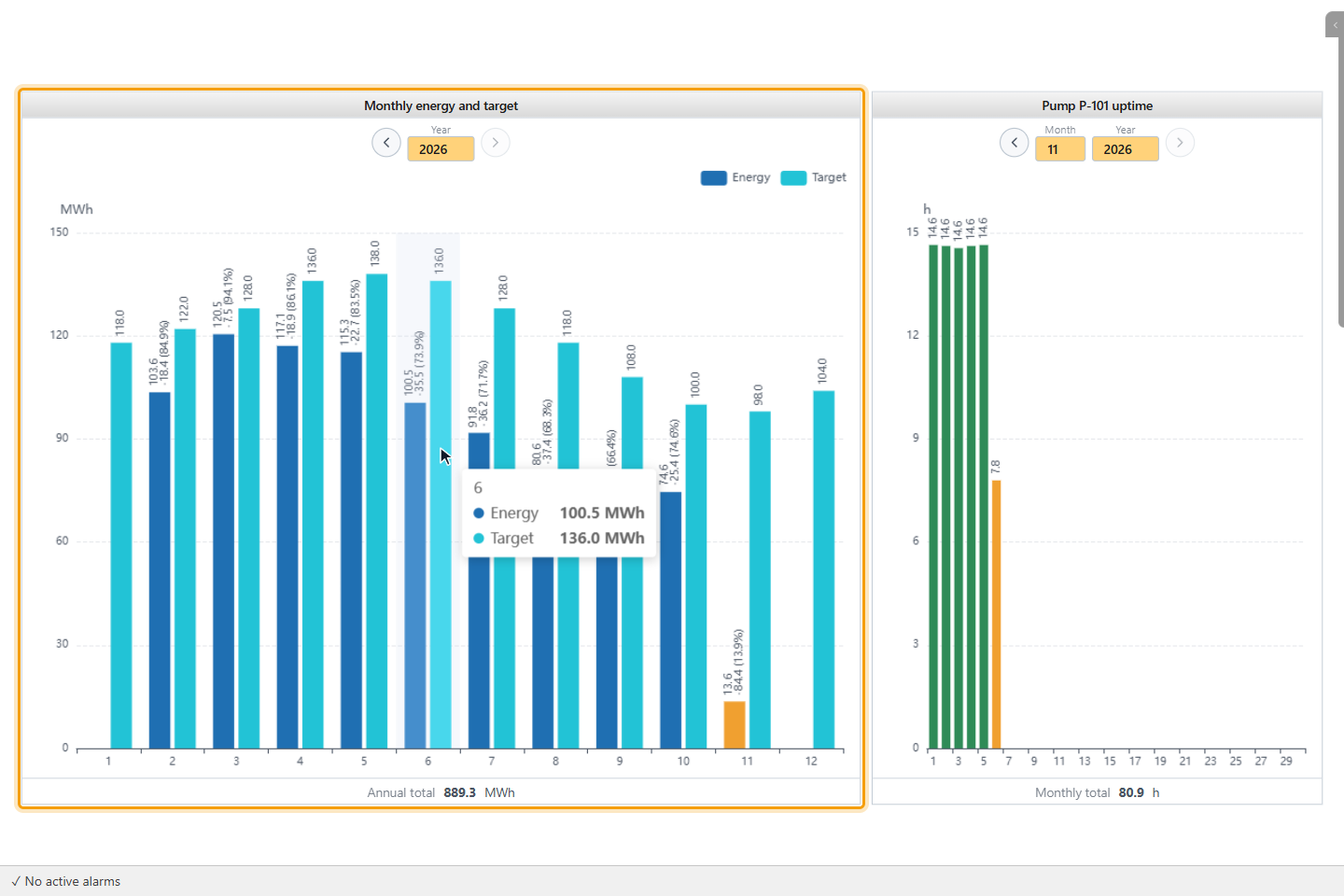
The bar of a running period has the Ongoing period color, and the object reads again every minute. A faded bar means that data is missing or that the meter was reset in this period. The line under the chart shows Daily total, Monthly total or Annual total for energy and uptime, and Average for the other measurements.
Data could not be retrieved means that a signal does not exist or that the history cannot be read. No signal selected means that Signals is empty.
5. Compare with the targets
In the monthly view, a second bar in the Target color stands next to each month. The label of the value bar shows the value, the difference from the target and the value as a percentage of the target.
6. Show the uptime (optional)
Set Measurement to Uptime and fill in the power and breaker fields. The unit is h. You can skip this step if you
do not need running hours.
7. Place an Analysis Chart
In WIDGETS, click Analysis Chart and draw a rectangle on the page. Choose the Chart type and add the pens under Signals. All fields are listed in Analysis Chart.
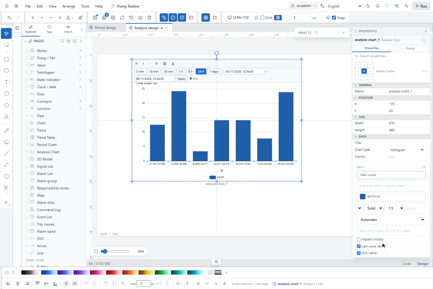
The chart types need these fields:
| Chart type | Signals used | More fields |
|---|---|---|
| Histogram | All | Number of bins: empty is automatic, 5 to 60 |
| Duration curve | All | Logarithmic axis |
| State timeline | All | Threshold (above = on): empty is a binary or integer state |
| Heatmap (day × hour) | The first | |
| Time comparison | All | Comparison (hours ago): 24 is yesterday, 168 is last week. Logarithmic axis |
| SPC control chart (I-MR) | The first | |
| Box plot (per day) | The first | |
| XY points, XY scatter (trend line + R²), XY line (trajectory) | One Y per pen | X-axis signal |
The time range is set as for a trend: Time mode with Live duration (min) (default 1440) or Start and End. On the run screen the object has the toolbar with the time buttons, Stop and Export, and the date-time bar; see Trend and Trend Table objects. The statistics are calculated from the averages of the intervals in the range, not from the raw samples. A longer range therefore has coarser values.
8. Read the distribution
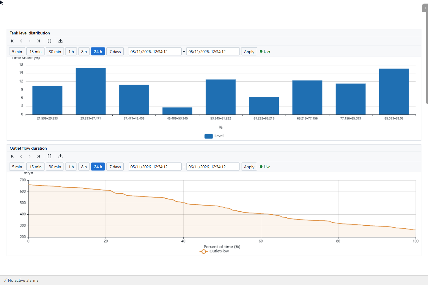
Histogram shows how much of the time (Time share (%)) the value was in each bin. Duration curve sorts the values from high to low over Percent of time (%): at 20 % you read the value that was exceeded in 20 % of the time.
9. Read states and daily patterns
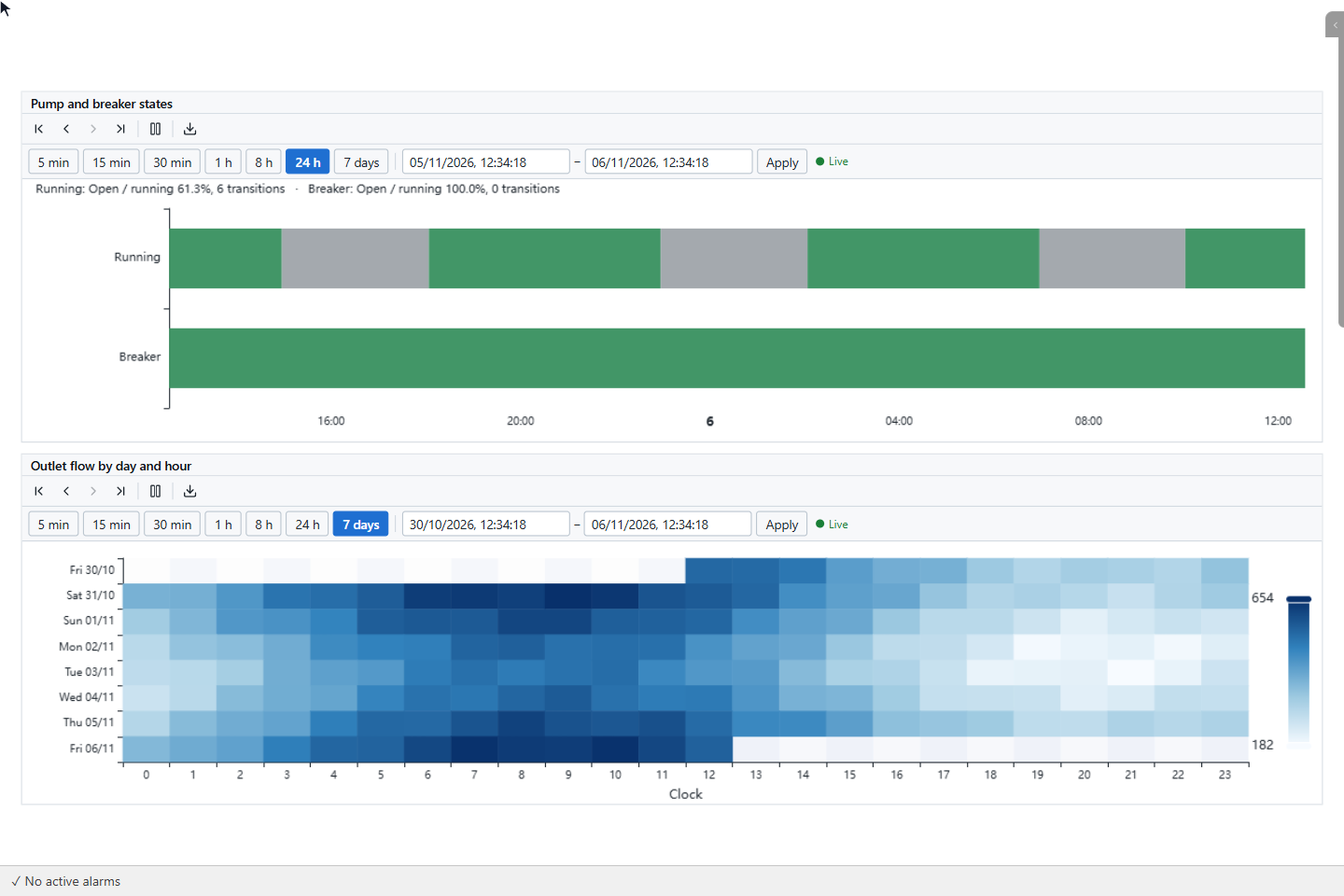
State timeline has a row per signal with a band for each state. The line above it gives the share of Open / running and the number of transitions. Heatmap (day × hour) shows the average of the first signal for each day (rows) and hour (columns, axis Clock), so a repeating daily pattern is visible at a glance.
10. Check the stability
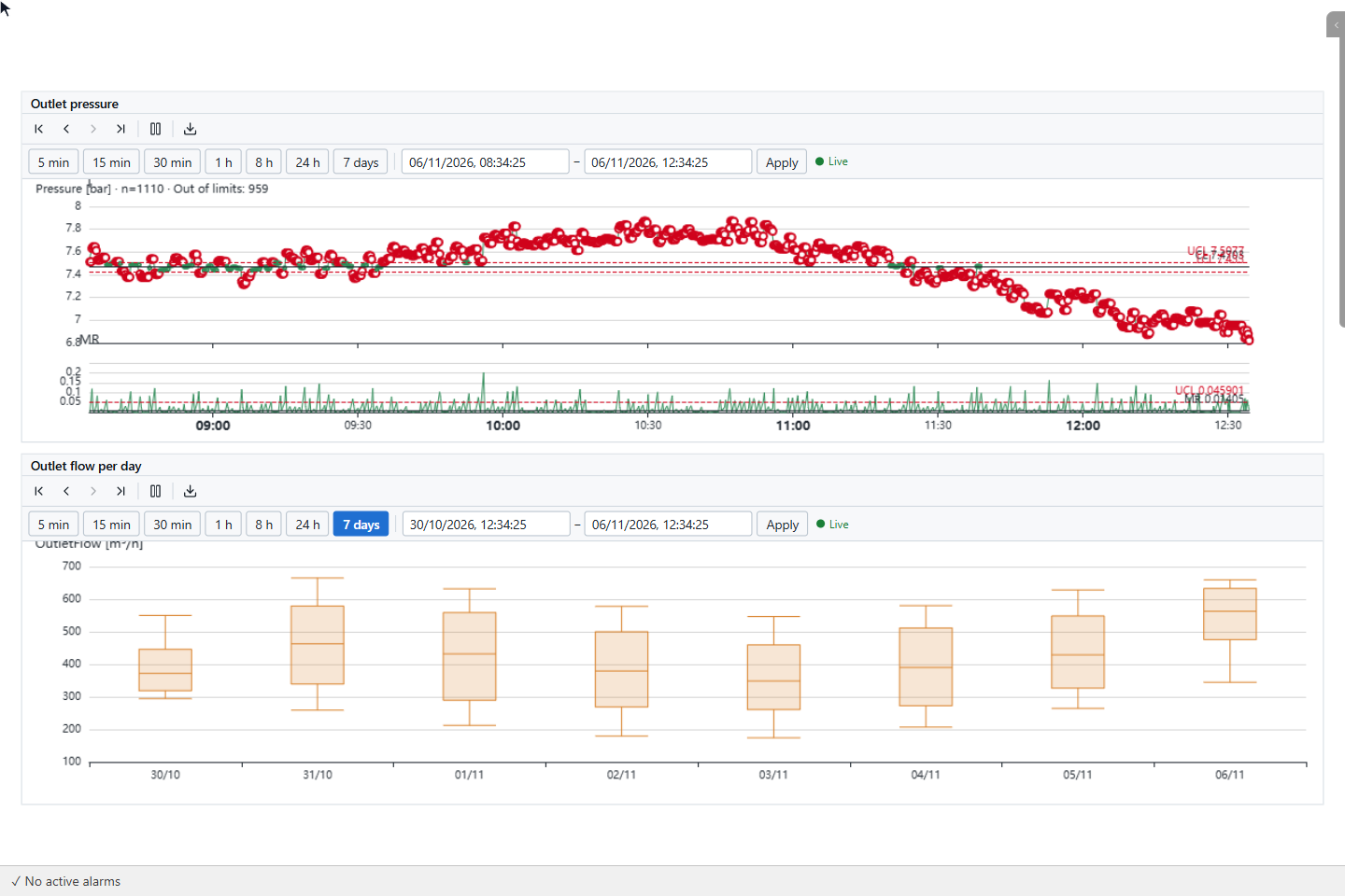
SPC control chart (I-MR) shows the values of the first signal with their mean and control limits, and below them the moving range. Points out of the limits are red; the title gives the number of values and of points Out of limits. Box plot (per day) draws one box per day with the median, the quartiles and the whiskers, and outliers in red.
11. Compare periods and signals
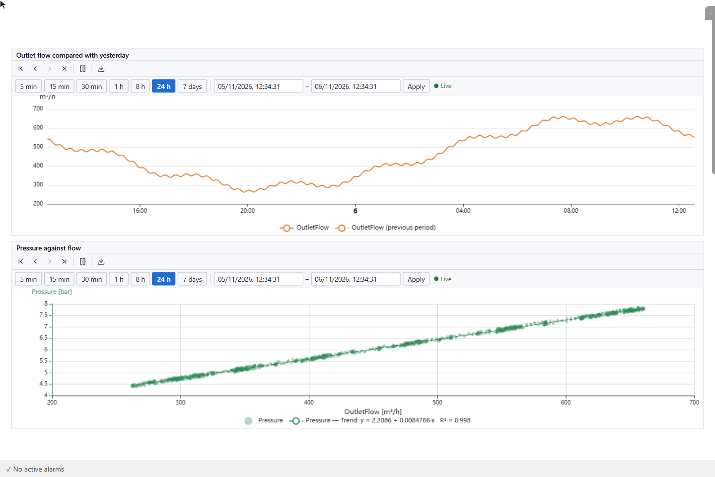
Time comparison draws the range and, dashed, the same range Comparison (hours ago) earlier; the legend calls it previous period. The XY charts draw one signal against another: YTCC pairs the values by time and leaves out pairs that are further apart than 30 seconds or two intervals, whichever is longer. XY scatter (trend line + R²) adds the trend line and its R². If the signals have no values at common times, the chart stays empty.
Next steps
- Trend and Trend Table objects show the values over time.
- Draw charts from the screen opens the same chart types for signals the operator clicks.
- Export data describes the files.